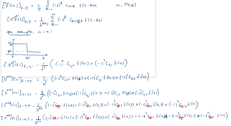
Considere a definição de GL, em que a ordem é variável no tempo
$\frac{d^{\alpha(t)} f(t)}{dt^{\alpha(t)}}=
\lim_{h\rightarrow 0^+} \frac{1}{h^{\alpha(t)}}
\sum_{k=0}^{N} (-1)^k C_{\alpha(t),k}^* f(t-kh)$
com $t\in [0,+\infty)$ e $\alpha \in \Re^+$. Onde $N=\lceil t/h\rceil$, i.e. $N$ é o maior inteiro próximo de $t/h$, isto garante que o menor $t$ que entra no somatório é $0$. Veja que para esta definição os coeficientes do passado são obtidos para a ordem calculada no tempo presente.
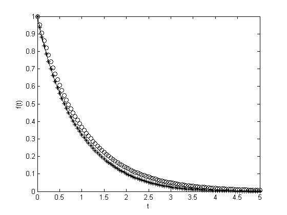
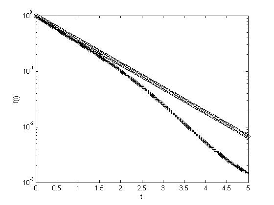
Considere o problema
$\frac{d^{\alpha(t)} f(t)}{dt^{\alpha(t)}}=-kf(t)$
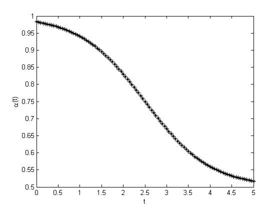
A figura abaixo mostra a ordem variável assumida durante o tempo. A seguir os resultados simulados para f0=1, tmax=5, h=0.05 e L=1 $($foi usado o programa com comprimento de memória$)$.
function vodfracL2
y0=1;
tmax=5;
h=0.05;
L=1;
global a
t=0:h:tmax;t=t';
y(1)=y0;
N=length(t);
NL=fix(L/h);
for j=2:N;
ai=1; af=.5; tcorte=tmax/2; v=1.5; alpha(1)=((tanh((0-tcorte)/v)+1)/2)*(af-ai)+ai;
a=((tanh((t(j)-tcorte)/v)+1)/2)*(af-ai)+ai;
c=(-1)^(j+1)*cbg(a,j)*y(1);
if j<NL
L1=j;
else
L1=NL;
end
for k=1:L1-1
c=c+(-1)^(k+1)*cbg(a,k)*y(j-k);
end
y(j)=c+h^a*func(y(end),t(j));
tempo(j)=t(j);
alpha(j)=a;
end
plot(tempo,alpha,'k*-')
xlabel('t')
ylabel('\alpha(t)')
figure
plot(tempo,y,'k*-',tempo,1*exp(-1*t),'ko')
xlabel('t')
ylabel('f(t)')
figure
semilogy(tempo,y,'k*-',tempo,1*exp(-1*t),'ko')
xlabel('t')
ylabel('f(t)')
end
function w=cbg(a,k)
w=1;
for j=1:k
w=w*(1-(a+1)/j);
end
w=w/(-1)^k;
end
function f=func(y,t)
global a
f=-1*y;
end